

Mastering Circuits!
Mastering the Methods of Analysis in Electrical Circuits is essential for everyone. Today, we are going to learn about essential techniques like Nodal Analysis, Nodal Analysis with Voltage Sources (Supernodes), Mesh Analysis, Mesh Analysis with Current Sources (Supermeshes). We will also solve some problems related to these topics. Learn these topics with Mastering Circuits.
Nodal Analysis
Steps for Nodal Analysis
1. Identify All Nodes
Locate all the connection points in the circuits. Specifically, identify the essential nodes, nodes where three or more circuit elements (resistors, sources, etc.) meet.

Figure 1 – Identifying all nodes
2. Select a Reference Node (Ground)
Choose one node to be the Reference Node, also known as the Ground. The voltage at this node is defined as 0 V. Usually, the node at the bottom of the circuit is chosen as the Reference.

Figure 2 – Common symbols for indicating a reference node (a) common ground, (b) ground, (c) chassis ground
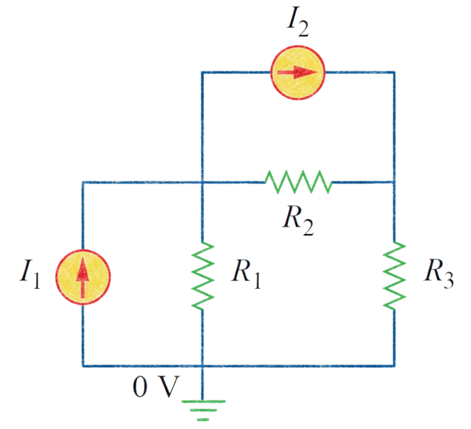
Figure 3 – Selecting a reference node (ground)
3. Assign Node Voltages
Label the remaining non-reference nodes as V1, V2, … , Vn. These are the unknown variables you need to solve for.
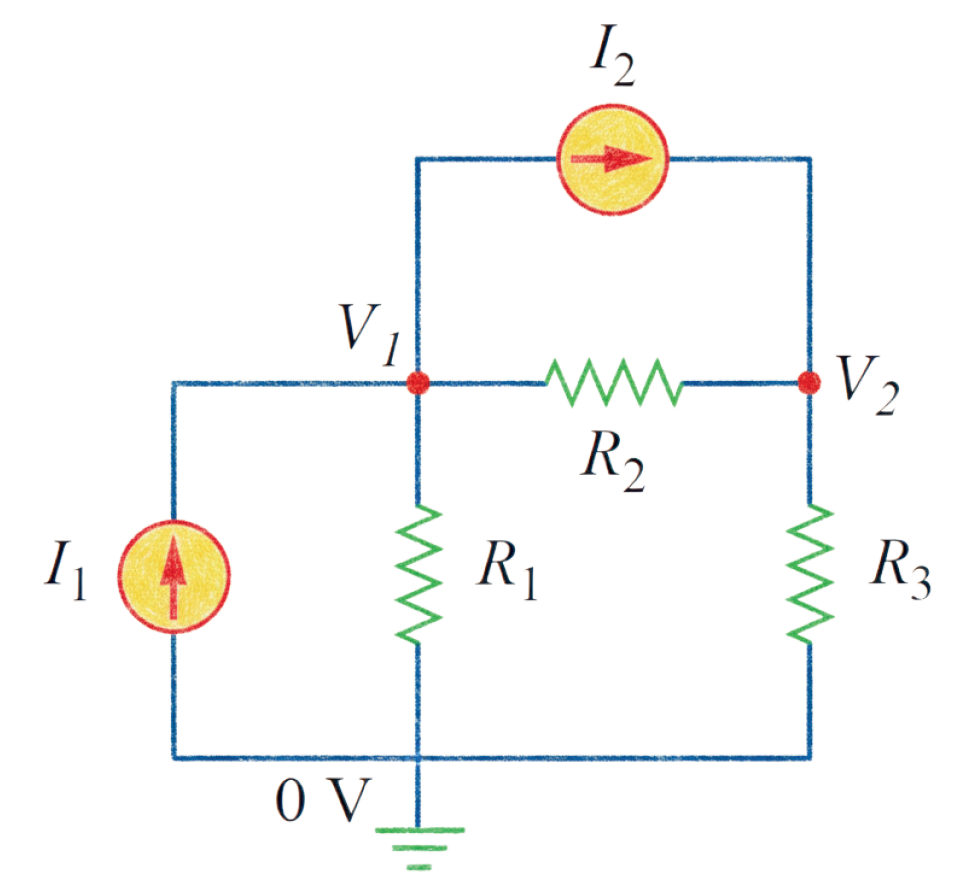
Figure 4 – Assigning node voltages
4. Apply Kirchhoff’s Current Law (KCL)
At each non-reference node, write a KCL equation. According to KCL, the algebraic sum of currents leaving a node must be zero.
- Express Currents using Ohm’s Law: For a branch with resistance R between two nodes, the current I is:
I = \frac{V_{higher} - V_{lower}}{R}
- Sign Convention:
- Positive (+): Currents leaving the node
- Negative (-): Currents entering the node

Figure 5 – Applying Kirchhoff’s Current Law (KCL)
\small \begin{aligned} & \text{KCL at node 1 in Fig. 5,} \\[2ex] & -I_1 + I_2 + \frac{V_1 - 0}{R_1} + \frac{V_1 - V_2}{R_2} = 0 \\[2ex] & \therefore -I_1 + I_2 + \frac{V_1}{R_1} + \frac{V_1 - V_2}{R_2} = 0 \\[4.5ex] & \text{KCL at node 2 in Fig. 5,} \\[2ex] & -I_2 + \frac{V_2 - 0}{R_3} + \frac{V_2 - V_1}{R_2} = 0 \\[2ex] & \therefore -I_2 + \frac{V_2}{R_3} + \frac{V_2 - V_1}{R_2} = 0 \end{aligned}
5. Solve the Equations
If you have n non-reference nodes, you will have n independent linear equations.
Solve for the unknown voltages (V1, V2, etc.).
\small \begin{aligned} & \text{Let,} \\[2ex] & \quad R_1 = 4 \ \Omega, \ R_2 = 2 \ \Omega, \ R_3 = 8 \ \Omega \\[2ex] & \quad I_1 = 5 \ A, \ I_2 = 2 \ A \end{aligned}

Figure 6 – Solving the equations
\small \begin{aligned} & \text{KCL at node 1 in Fig. 6,} \\[2ex] & -5 + 2 + \frac{V_1}{4} + \frac{V_1 - V_2}{2} = 0 \\[2ex] & \Rightarrow \frac{V_1 + 2V_1 - 2V_2}{4} = 3 \\[2ex] & \therefore 3V_1 - 2V_2 = 12 \quad \text{\text{-} \text{-} \text{-} (i)} \\[3ex] & \text{KCL at node 2 in Fig. 6,} \\[2ex] & -2 + \frac{V_2 - V_1}{2} + \frac{V_2}{8} = 0 \\[2ex] & \Rightarrow \frac{4V_2 - 4V_1 + V_2}{8} = 2 \\[2ex] & \therefore -4V_1 + 5V_2 = 16 \quad \text{\text{-} \text{-} \text{-} (ii)} \\[3ex] & \text{Solving the equations (i) \& (ii),} \\[2.5ex] & \therefore V_1 = 13.14 \ V, \ V_2 = 13.71 \ V \end{aligned}
Solved Problems on Nodal Analysis
Problem 1
Pb-1: Calculate the node voltages in the circuit shown in Fig. 7.

Figure 7 – Circuit diagram for Pb-1
Solution:

Figure 8 – Circuit diagram for solving the Pb-1
\small \begin{aligned} & \text{KCL at node 1,} \\[2ex] & -5 + \frac{v_1}{2} + \frac{v_1 - v_2}{4} = 0 \\[2ex] & \Rightarrow \frac{-20 + 2v_1 + v_1 - v_2}{4} = 0 \\[2ex] & \therefore 3v_1 - v_2 = 20 \quad \text{\text{-} \text{-} \text{-} (i)} \\[3ex] & \text{KCL at node 2,} \\[2ex] & -10 + 5 + \frac{v_2}{6} + \frac{v_2 - v_1}{4} = 0 \\[2ex] & \Rightarrow \frac{-60 + 2v_2 + 3v_2 - 3v_1}{12} = 0 \\[2ex] & \therefore -3v_1 + 5v_2 = 60 \quad \text{\text{-} \text{-} \text{-} (ii)} \\[3ex] & \text{Solving equations (i) \& (ii),} \\[2.5ex] & \therefore v_1 = 13.33 \ V, \ v_2 = 20 \ V \end{aligned}
Problem 2
Pb-2: Obtain the node voltages in the circuit of Fig. 9.

Figure 9 – Circuit diagram for Pb-2
Solution:

Figure 10 – Circuit diagram for solving the Pb-2
\small \begin{aligned} &\text{KCL at node 1,} \\[2ex] & -3 + \frac{v_1}{2} + \frac{v_1 - v_2}{6} = 0 \\[2ex] & \Rightarrow \frac{-18 + 3v_1 + v_1 - v_2}{6} = 0 \\[2ex] & \therefore 4v_1 - v_2 = 18 \quad \text{\text{-} \text{-} \text{-} (i)} \\[3ex] &\text{KCL at node 2,} \\[2ex] & 12 + \frac{v_2}{7} + \frac{v_2 - v_1}{6} = 0 \\[2ex] & \Rightarrow \frac{504 + 6v_2 + 7v_2 - 7v_1}{42} = 0 \\[2ex] & \therefore -7v_1 + 13v_2 = -504 \quad \text{\text{-} \text{-} \text{-} (ii)} \\[3ex] &\text{Solving equations (i) \& (ii),} \\[2.5ex] & \therefore v_1 = -6 \ V, \ v_2 = -42 \ V \end{aligned}
Problem 3
Pb-3: Determine the voltages at the nodes in Fig. 11.

Figure 11 – Circuit diagram for Pb-3
Solution:

Figure 12 – Circuit diagram for solving the Pb-3
\small \begin{aligned} &\text{KCL at node 1,} \\[2ex] & -3 + \frac{v_1 - v_2}{2} + \frac{v_1 - v_3}{4} = 0 \\[2ex] & \Rightarrow \frac{-12 + 2v_1 - 2v_2 + v_1 - v_3}{4} = 0 \\[2ex] & \therefore 3v_1 - 2v_2 - v_3 = 12 \quad \text{\text{-} \text{-} \text{-} (i)} \\[3ex] & \text{KCL at node 2,} \\[2ex] & \frac{v_2}{4} + \frac{v_2 - v_1}{2} + \frac{v_2 - v_3}{8} = 0 \\[2ex] & \Rightarrow \frac{2v_2 + 4v_2 - 4v_1 + v_2 - v_3}{8} = 0 \\[2ex] & \therefore -4v_1 + 7v_2 - v_3 = 0 \quad \text{\text{-} \text{-} \text{-} (ii)} \\[3ex] &\text{KCL at node 3,} \\[2ex] & 2i_x + \frac{v_3 - v_1}{4} + \frac{v_3 - v_2}{8} = 0 \\[2ex] & \Rightarrow 2 \cdot \frac{v_1 - v_2}{2} + \frac{v_3 - v_1}{4} + \frac{v_3 - v_2}{8} = 0 \\[2ex] & \Rightarrow \frac{8v_1 - 8v_2 + 2v_3 - 2v_1 + v_3 - v_2}{8} = 0 \\[2ex] & \therefore 6v_1 - 9v_2 + 3v_3 = 0 \quad \text{\text{-} \text{-} \text{-} (iii)} \\[3.5ex] &\text{Solving equations (i), (ii) \& (iii),} \\[2.5ex] & \therefore v_1 = 4.8 \ V, \ v_2 = 2.4 \ V, \ v_3 = -2.4 \ V \end{aligned}
Problem 4
Pb-4: Find the voltages at the three non-reference nodes in the circuit of Fig. 13.

Figure 13 – Circuit diagram for Pb-4
Solution:

Figure 14 – Circuit diagram for solving the Pb-4
\small \begin{aligned} &\text{KCL at node 1,} \\[2ex] & -4 + \frac{v_1 - v_2}{3} + \frac{v_1 - v_3}{2} = 0 \\[2ex] & \Rightarrow \frac{-24 + 2v_1 - 2v_2 + 3v_1 - 3v_3}{6} = 0 \\[2ex] & \therefore 5v_1 - 2v_2 - 3v_3 = 24 \quad \text{\text{-} \text{-} \text{-} (i)} \\[3ex] &\text{KCL at node 2,} \\[2ex] & \frac{v_2}{4} + \frac{v_2 - v_1}{3} - 4i_x = 0 \\[2ex] & \Rightarrow \frac{v_2}{4} + \frac{v_2 - v_1}{3} - 4 \cdot \frac{v_2}{4} = 0 \\[2ex] & \Rightarrow \frac{3v_2 + 4v_2 - 4v_1 - 12v_2}{12} = 0 \\[2ex] & \therefore -4v_1 - 5v_2 = 0 \quad \text{\text{-} \text{-} \text{-} (ii)} \\[3ex] &\text{KCL at node 3,} \\[2ex] & \frac{v_3}{6} + \frac{v_3 - v_1}{2} + 4i_x = 0 \\[2ex] & \Rightarrow \frac{v_3}{6} + \frac{v_3 - v_1}{2} + 4 \cdot \frac{v_2}{4} = 0 \\[2ex] & \Rightarrow \frac{v_3 + 3v_3 - 3v_1 + 6v_2}{6} = 0 \\[2ex] & \therefore -3v_1 + 6v_2 + 4v_3 = 0 \quad \text{\text{-} \text{-} \text{-} (iii)} \\[3ex] &\text{Solving equations (i), (ii) \& (iii),} \\[2ex] & \therefore v_1 = 32 \ V, \ v_2 = -25.6 \ V, \ v_3 = 62.4 \ V \end{aligned}
Nodal Analysis (Super Node)
Steps for Nodal Analysis with Voltage Sources
1. Identify the SuperNode
Locate any voltage source (independent or dependent) that is connected between two non-reference nodes. Encircle this voltage source and the two nodes it connects to form a single, larger node.

Figure 15 – A circuit with a supernode
2. Write the Voltage Source Equation
The voltage source provides a direct relationship between the two nodes. Write an equation that defines this relationship:
V_{positive} - V_{negative} = V_{source}

Figure 16 – Defining the voltage source equation
\small \begin{aligned} &\text{The voltage source equation,} \\[1.5ex] & \quad \quad \quad \quad \therefore v_2 - v_3 = 5 \quad \text{\text{-} \text{-} \text{-} (i)} \end{aligned}
3. Apply KCL to the SuperNode
Treat the entire supernode boundary as one single node. Apply Kirchhoff’s Current Law (KCL) to the Node.
- Ignore the internal voltage source while writing the KCL equation.
- Sum the currents flowing through all resistors connected to either of the two nodes forming the supernode
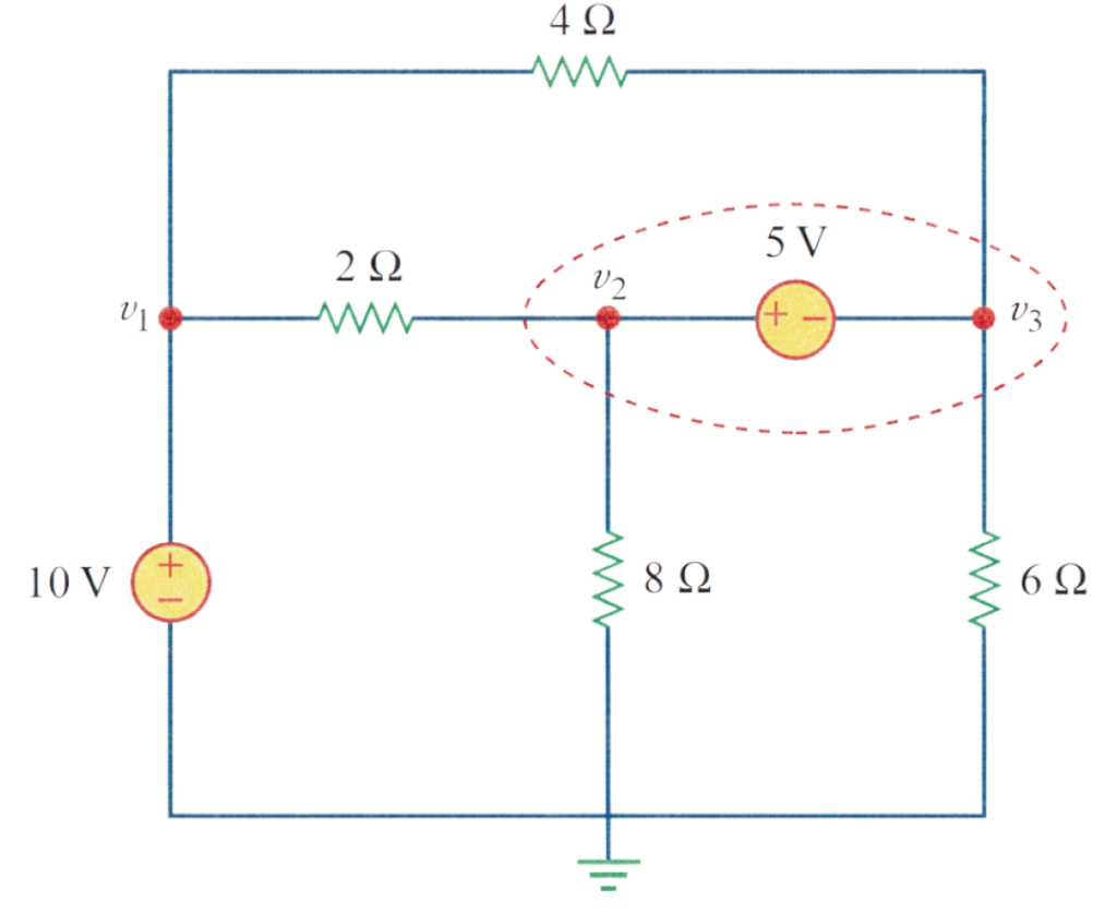
Figure 17 – Applying KCL to the SuperNode
\small \begin{aligned} &\text{KCL at SuperNode,} \\[2ex] & \frac{v_2}{8} + \frac{v_2 - v_1}{2} + \frac{v_3}{6} + \frac{v_3 - v_1}{4} = 0 \\[2ex] & \Rightarrow \frac{v_2}{8} + \frac{v_2 - 10}{2} + \frac{v_3}{6} + \frac{v_3 - 10}{4} = 0 \\[2ex] & \Rightarrow \frac{3v_2 + 12v_2 - 120 + 4v_3 + 6v_3 - 60}{24} = 0 \\[2ex] & \therefore 15v_2 + 10v_3 = 180 \quad \text{\text{-} \text{-} \text{-} (ii)} \end{aligned}
4. Apply KCL to Remaining Nodes
If there are other non-reference nodes in the circuit that are not part of a supernode, write standard KCL equations for them as usual.

Figure 18 – Applying KCL to the Remaining Nodes
From Fig. 18, we can see that v_{1} = 10 \ V . So we don’t need to apply KCL here to find the node voltage (v_{1}) .
\small \begin{aligned} & \quad \quad \quad \quad \therefore v_1 = 10 \quad \text{\text{-} \text{-} \text{-} (iii)} \end{aligned}
5. Solve the System of Equations
Combine the voltage source equation and all the KCL equations to solve for all unknown node voltages.
\small \begin{aligned} &\text{The equations,} \\[2ex] & \quad v_2 - v_3 = 5 \quad \text{\text{-} \text{-} \text{-} (i)} \\[2ex] & \quad 15v_2 + 10v_3 = 180 \quad \text{\text{-} \text{-} \text{-} (ii)} \\[2ex] & \quad v_1 = 10 \quad \text{\text{-} \text{-} \text{-} (iii)} \\[3ex] &\text{Solving equations (i), (ii) and (iii),} \\[2.5ex] & \therefore v_1 = 10 \ V, \ v_2 = 9.2 \ V, \ v_3 = 4.2 \ V \end{aligned}
Solved Problems on Nodal Analysis (Super Node)
Problem 5
Pb-5: For the circuit shown in Fig. 19, find the node voltages.

Figure 19 – Circuit diagram for Pb-5
Solution:

Figure 20 – Circuit diagram for solving the Pb-5
\small \begin{aligned} &\text{The voltage source equation,} \\[2ex] & v_2 - v_1 = 2 \\[2ex] & \therefore -v_1 + v_2 = 2 \quad \text{\text{-} \text{-} \text{-} (i)} \\[3ex] &\text{KCL at SuperNode,} \\[2ex] & -2 + \frac{v_1}{2} + \frac{v_2}{4} + 7 = 0 \\[2ex] & \Rightarrow \frac{-8 + 2v_1 + v_2 + 28}{4} = 0 \\[2ex] & \therefore 2v_1 + v_2 = -20 \quad \text{\text{-} \text{-} \text{-} (ii)} \\[3.5ex] &\text{Solving equations (i) and (ii),} \\[2.5ex] & \therefore v_1 = -7.33 \ V, \ v_2 = -5.33 \ V \end{aligned}
Problem 6
Pb-6: Find v and i in the circuit of Fig. 21.

Figure 21 – Circuit diagram for Pb-6
Solution:

Figure 22 – Circuit diagram for solving the Pb-6
\small \begin{aligned} &\text{The voltage source equation,} \\[2ex] & v_2 - v_1 = 6 \\[2ex] & \therefore -v_1 + v_2 = 6 \quad \text{\text{-} \text{-} \text{-} (i)} \\[3ex] &\text{KCL at SuperNode,} \\[2ex] & \frac{v_1 - 14}{4} + \frac{v_1}{3} + \frac{v_2}{2} + \frac{v_2}{6} = 0 \\[2ex] & \Rightarrow \frac{3v_1 - 42 + 4v_1 + 6v_2 + 2v_2}{12} = 0 \\[2ex] & \therefore 7v_1 + 12v_2 = 42 \quad \text{\text{-} \text{-} \text{-} (ii)} \\[3ex] &\text{Solving equations (i) and (ii),} \\[2.5ex] & \therefore v_1 = -0.4 \ V, \quad v_2 = 5.6 \ V \\[2ex] & \therefore v = v_1 = -0.4 \ V = -400 \ mV \\[2ex] & \& \ i = \frac{v_2}{2} = \frac{5.6}{2} = 2.8 \ A \end{aligned}
Problem 7
Pb-7: Find the node voltages in the circuit of Fig. 23.

Figure 23 – Circuit diagram for Pb-7
Solution:

Figure 24 – Circuit diagram for solving the Pb-7
\small \begin{aligned} &\text{The voltage source equation (for } 20 \ V \text{),} \\[2ex] & \therefore v_1 - v_2 = 20 \quad \text{\text{-} \text{-} \text{-} (i)} \\[3ex] &\text{The voltage source equation (for } 3v_x \text{),} \\[2ex] & v_3 - v_4 = 3v_x = 3(v_1 - v_4) \\[2ex] & \Rightarrow v_3 - v_4 = 3v_1 - 3v_4 \\[2ex] & \therefore 3v_1 - v_3 - 2v_4 = 0 \quad \text{\text{-} \text{-} \text{-} (ii)} \\[3ex] &\text{KCL at SuperNode (for node 1 \& 2),} \\[2ex] &\frac{v_1}{2} + \frac{v_1 - v_4}{3} - 10 + \frac{v_2 - v_3}{6} = 0 \\[2ex] & \Rightarrow \frac{3v_1 + 2v_1 - 2v_4 - 60 + v_2 - v_3}{6} = 0 \\[2ex] & \therefore 5v_1 + v_2 - v_3 - 2v_4 = 60 \quad \text{\text{-} \text{-} \text{-} (iii)} \\[3.5ex] & \text{KCL at SuperNode (for node 3 \& 4),} \\[2ex] & \frac{v_4}{1} + \frac{v_4 - v_1}{3} + \frac{v_3}{4} + \frac{v_3 - v_2}{6} = 0 \\[2ex] & \Rightarrow \frac{24v_4 + 8v_4 - 8v_1 + 6v_3 + 4v_3 - 4v_2}{24} = 0 \\[2ex] & \therefore -8v_1 - 4v_2 + 10v_3 + 32v_4 = 0 \quad \text{\text{-} \text{-} \text{-} (iv)} \\[3ex] &\text{Solving equations (i), (ii), (iii) and (iv),} \\[2.5ex] & \therefore v_1 = 26.67 \ V, \ v_2 = 6.67 \ V, \\[2ex] & \quad \, v_3 = 173.33 \ V, \ v_4 = -46.67 \ V \end{aligned}
Problem 8
Pb-8: Find v_1, v_2, and v_3 in the circuit of Fig. 25 using nodal analysis.

Figure 25 – Circuit diagram for Pb-8
Solution:

Figure 26 – Circuit diagram for solving the Pb-8
\small \begin{aligned} & \text{The voltage source equation (for } 25 \ V \text{),} \\[2ex] & \therefore v_1 - v_2 = 25 \quad \text{\text{-} \text{-} \text{-} (i)} \\[3ex] &\text{The voltage source equation (for } 5i \text{),} \\[2ex] & v_3 - v_2 = 5i = 5 \cdot \frac{v_1}{2} \\[2ex] & \Rightarrow 2v_3 - 2v_2 = 5v_1 \\[2ex] & \therefore 5v_1 + 2v_2 - 2v_3 = 0 \quad \text{\text{-} \text{-} \text{-} (ii)} \\[3ex] &\text{KCL at SuperNode,} \\[2ex] & \frac{v_1}{2} + \frac{v_2}{4} + \frac{v_3}{3} = 0 \\[2ex] & \Rightarrow \frac{6v_1 + 3v_2 + 4v_3}{12} = 0 \\[2ex] & \therefore 6v_1 + 3v_2 + 4v_3 = 0 \quad \text{\text{-} \text{-} \text{-} (iii)} \\[3ex] &\text{Solving equations (i), (ii) and (iii),} \\[2.5ex] & \therefore v_1 = 7.608 \ V, \ v_2 = -17.39 \ V, \ v_3 = 1.63 \ V \end{aligned}
Mesh Analysis
Planar Circuits: A planar circuit is a circuit that can be drawn on a plane (a flat 2D surface) such that no two branches (wires) cross each other.

Figure 27 – (a) A planar circuit with crossing branches, (b) the same circuit redrawn with no crossing branches
Non-Planar Circuits: A non-planar circuit is a circuit that cannot be drawn on a plane without at least two branches crossing over one another.

Figure 28 – A non-planar circuit
Mesh Analysis is only applicable for Planar Circuit.
Steps for Mesh Analysis
1. Identify the Meshes
Count the total number of meshes in the circuit. A mesh is a loop that does not contain any other loops within it.

Figure 29 – Identifying the meshes
2. Assign Mesh Currents
Assign a unique current variable (e.g. i_{1}, i_{2}, i_{3}) to each other.
- Direction: For consistency, it is best to assign all mesh currents in the clockwise direction. This simplifies the math and reduces sign errors.

Figure 30 – Assigning mesh currents
3. Label the Polarity of Resistors
As the mesh current flows through a resistor, it creates a voltage drop.
- Mark the side where the current enters the resistor as positive (+) and the side where it leaves as negative (-).
- For resistors shared between two meshes, the polarity will depend on which mesh is currently being analyzed.

Figure 31 – Labeling the polarity of resistors
4. Apply Kirchhoff’s Voltage Law (KVL)
At each mesh, write a KVL equation. According to KVL, the algebraic sum of voltages around a closed loop must be zero.
- Express Voltages using Ohm’s Law: The voltage across a resistor is the product of the mesh current and the resistance (V = iR) .
- Shared Branches: If a resistor is shared between two meshes (e.g. Mesh 1 and Mesh 2), the net current through it is (i_{1} - i_{2}) if Mesh 1 is being analyzed.

Figure 32 – Applying Kirchhoff’s Voltage Law (KVL)
\small \begin{aligned} &\text{KVL at mesh 1,} \\[2ex] & -V_1 + i_1 R_1 + (i_1 - i_2)R_3 = 0 \\[2ex] & \therefore -V_1 + i_1 R_1 + i_1 R_3 - i_2 R_3 = 0 \\[3ex] &\text{KVL at mesh 2,} \\[2ex] & (i_2 - i_1)R_3 + i_2 R_2 + V_2 = 0 \\[2ex] & \therefore i_2 R_3 - i_1 R_3 + i_2 R_2 + V_2 = 0 \end{aligned}
5. Solve the Equations
If you have n meshes, you will have n independent linear equations.
Solve for the unknown currents (i1, i2, etc.).
\small \begin{aligned} & \text{Let,} \\[2ex] & \quad R_1 = 2 \ \Omega, \ R_2 = 4 \ \Omega, \ R_3 = 6 \ \Omega \\[2ex] & \quad V_1 = 12 \ V, \ V_2 = 10 \ V \end{aligned}

Figure 33 – Solving the equations
\small \begin{aligned} &\text{KVL at mesh 1,} \\[2ex] & -12 + 2i_1 + 6(i_1 - i_2) = 0 \\[2ex] & \Rightarrow 2i_1 + 6i_1 - 6i_2 = 12 \\[2ex] & \therefore 8i_1 - 6i_2 = 12 \quad \text{\text{-} \text{-} \text{-} (i)} \\[3ex] &\text{KVL at mesh 2,} \\[2ex] & 6(i_2 - i_1) + 4i_2 + 10 = 0 \\[2ex] & \Rightarrow 6i_2 - 6i_1 + 4i_2 = -10 \\[2ex] & \therefore -6i_1 + 10i_2 = -10 \quad \text{\text{-} \text{-} \text{-} (ii)} \\[3ex] &\text{Solving the equations (i) \& (ii),} \\[2ex] & \therefore i_1 = 1.36 \ A, \ i_2 = -0.18 \ A \end{aligned}
Solved Problems on Mesh Analysis
Problem 9
Pb-9: For the circuit in Fig. 34, find the branch currents I_{1}, I_{2} and I_3 using mesh analysis.

Figure 34 – Circuit diagram for Pb-9
Solution:

Figure 35 – Circuit diagram for solving the Pb-9
\small \begin{aligned} &\text{KVL at mesh 1,} \\[2ex] & -15 + 5i_1 + 10(i_1 - i_2) + 10 = 0 \\[2ex] & \Rightarrow -5 + 5i_1 + 10i_1 - 10i_2 = 0 \\[2ex] & \therefore 15i_1 - 10i_2 = 5 \quad \text{\text{-} \text{-} \text{-} (i)} \\[3ex] &\text{KVL at mesh 2,} \\[2ex] & -10 + 10(i_2 - i_1) + 6i_2 + 4i_2 = 0 \\[2ex] & \Rightarrow 10i_2 - 10i_1 + 6i_2 + 4i_2 = 10 \\[2ex] & \therefore -10i_1 + 20i_2 = 10 \quad \text{\text{-} \text{-} \text{-} (ii)} \\[3ex] &\text{Solving equations (i) and (ii),} \\[2ex] & \therefore i_1 = 1 \ A, \ i_2 = 1 \ A \\[2ex] & \therefore I_1 = i_1 = 1 \ A, \ I_2 = i_2 = 1 \ A \\[3ex] &\text{KCL at node a,} \\[2ex] & I_3 + I_2 - I_1 = 0 \\[2ex] & \Rightarrow I_3 + 1 - 1 = 0 \\[2ex] & \therefore I_3 = 0 \ A \end{aligned}
Problem 10
Pb-10: Calculate the mesh currents i_1 and i_2 of the circuit of Fig. 36.

Figure 36 – Circuit diagram for Pb-10
Solution:

Figure 37 – Circuit diagram for solving the Pb-10
\small \begin{aligned} & \text{KVL at mesh 1,} \\[2ex] & -45 + 2i_1 + 12(i_1 - i_2) + 4i_1 = 0 \\[2ex] & \Rightarrow 2i_1 + 12i_1 - 12i_2 + 4i_1 = 45 \\[2ex] & \therefore 18i_1 - 12i_2 = 45 \quad \text{\text{-} \text{-} \text{-} (i)} \\[3ex] & \text{KVL at mesh 2,} \\[2ex] & 12(i_2 - i_1) + 9i_2 + 30 + 3i_2 = 0 \\[2ex] & \Rightarrow 12i_2 - 12i_1 + 9i_2 + 3i_2 = -30 \\[2ex] & \therefore -12i_1 + 24i_2 = -30 \quad \text{\text{-} \text{-} \text{-} (ii)} \\[3ex] & \text{Solving equations (i) and (ii),} \\[2ex] & \therefore i_1 = 2.5 \ A, \quad i_2 = 0 \ A \end{aligned}
Problem 11
Pb-11: Use mesh analysis to find the current I_0 in the circuit of Fig. 38.

Figure 38 – Circuit diagram for Pb-11
Solution:

Figure 39 – Circuit diagram for solving the Pb-11
\small \begin{aligned} &\text{KVL at mesh 1,} \\[2ex] & -24 + 10(i_1 - i_2) + 12(i_1 - i_3) = 0 \\[2ex] & \Rightarrow 10i_1 - 10i_2 + 12i_1 - 12i_3 = 24 \\[2ex] & \therefore 22i_1 - 10i_2 - 12i_3 = 24 \quad \text{\text{-} \text{-} \text{-} (i)} \\[3ex] &\text{KVL at mesh 2,} \\[2ex] & 10(i_2 - i_1) + 24i_2 + 4(i_2 - i_3) = 0 \\[2ex] & \Rightarrow 10i_2 - 10i_1 + 24i_2 + 4i_2 - 4i_3 = 0 \\[2ex] & \therefore -10i_1 + 38i_2 - 14i_3 = 0 \quad \text{\text{-} \text{-} \text{-} (ii)} \\[3.5ex] &\text{KCL at node A,} \\[2ex] & i_2 + I_0 - i_1 = 0 \\[2ex] & \therefore I_0 = i_1 - i_2 \\[3ex] &\text{KVL at mesh 3,} \\[2ex] & 12(i_3 - i_1) + 4(i_3 - i_2) + 4I_0 = 0 \\[2ex] & \Rightarrow 12i_3 - 12i_1 + 4i_3 - 4i_2 + 4(i_1 - i_2) = 0 \\[2ex] & \Rightarrow 12i_3 - 12i_1 + 4i_3 - 4i_2 + 4i_1 - 4i_2 = 0 \\[2ex] & \therefore -8i_1 - 8i_2 + 16i_3 = 0 \quad \text{\text{-} \text{-} \text{-} (iii)} \\[3ex] &\text{Solving equations (i), (ii) and (iii),} \\[2ex] & \therefore i_1 = 2.25 \ A, \ i_2 = 0.75 \ A, \ i_3 = 1.5 \ A \\[2ex] & I_0 = i_1 - i_2 = 2.25 - 0.75 \\[2ex] & \therefore I_0 = 1.5 \ A \end{aligned}
Problem 12
Pb-12: Using mesh analysis, find i_0 in the circuit of Fig. 40.

Figure 40 – Circuit diagram for Pb-12
Solution:

Figure 41 – Circuit diagram for solving the Pb-12
\small \begin{aligned} &\text{KVL at mesh 1,} \\[2ex] & -16 + 4(i_1 - i_3) + 2(i_1 - i_2) = 0 \\[2ex] & \Rightarrow 4i_1 - 4i_3 + 2i_1 - 2i_2 = 16 \\[2ex] & \therefore 6i_1 - 2i_2 - 4i_3 = 16 \quad \text{\text{-} \text{-} \text{-} (i)} \\[3ex] & \text{KVL at mesh 3,} \\[2ex] & 4(i_3 - i_1) + 6i_3 + 8(i_3 - i_2) = 0 \\[2ex] & \Rightarrow 4i_3 - 4i_1 + 6i_3 + 8i_3 - 8i_2 = 0 \\[2ex] & \therefore -4i_1 - 8i_2 + 18i_3 = 0 \quad \text{\text{-} \text{-} \text{-} (ii)} \\[3ex] &\text{KVL at mesh 2,} \\[2ex] & 2(i_2 - i_1) + 8(i_2 - i_3) - 10i_0 = 0 \\[2ex] & \Rightarrow 2i_2 - 2i_1 + 8i_2 - 8i_3 - 10i_3 = 0 \\[2ex] & \therefore -2i_1 + 10i_2 - 18i_3 = 0 \quad \text{\text{-} \text{-} \text{-} (iii)} \\[3ex] &\text{Solving equations (i), (ii) and (iii),} \\[2ex] & \therefore i_1 = -2.57 \ A, \ i_2 = -7.71 \ A, \ i_3 = -4 \ A \\[2ex] & \therefore i_0 = i_3 = -4 \ A \end{aligned}
Mesh Analysis (Super Mesh)
1. Identify the Meshes
Locate any current source (independent or dependent) that is shared between two meshes. Encircle the shared branch, including the current source and any components in series with it.
SuperMesh is formed by removing the branch containing the current source (and any components in series with it), and treating the two meshes as a single, larger loop.

Figure 42 – Identifying the supermesh
2. Apply KCL at a Shared Node
Identify the two nodes where the shared current source is connected. Apply Kirchhoff’s Current Law (KCL) at either one of these nodes.

Figure 43 – Applying KCL at a shared node
\small \begin{aligned} &\text{KCL at node a,} \\[2ex] & i_1 - i_2 + 6 = 0 \\[2ex] & \therefore i_1 - i_2 = -6 \quad \text{\text{-} \text{-} \text{-} (i)} \end{aligned}
3. Apply KVL to the SuperMesh
Apply Kirchhoff’s Voltage Law (KVL) to the large outer loop that encloses both meshes.
- Ignore the shared branch, including the current source and any components in series with it while writing the KVL equation.
- Sum the voltage drops across all resistors and any voltage sources located in the supermesh.

Figure 44 – Applying KVL to the supermesh
\small \begin{aligned} &\text{KVL at SuperMesh,} \\[2ex] & -20 + 6i_1 + 10i_2 + 4(i_2 - i_3) = 0 \\[2ex] & \Rightarrow 6i_1 + 10i_2 + 4i_2 - 4i_3 = 20 \\[2ex] & \therefore 6i_1 + 14i_2 - 4i_3 = 20 \quad \text{\text{-} \text{-} \text{-} (ii)} \end{aligned}
4. Apply KVL to Remaining Meshes
If there are other meshes in the circuit that are not part of a supermesh, write standard KVL equations for them as usual.

Figure 45 – Applying KVL to remaining meshes
\small \begin{aligned} &\text{KVL at mesh 3,} \\[2ex] & 4(i_3 - i_2) + 8i_3 - 10 = 0 \\[2ex] & \Rightarrow 4i_3 - 4i_2 + 8i_3 = 10 \\[2ex] & \therefore -4i_2 + 12i_3 = 10 \quad \text{\text{-} \text{-} \text{-} (iii)} \end{aligned}
5. Solve the System of Equations
Combine the KCL equation and all the KVL equations to solve for all unknown mesh currents.
\small \begin{aligned} &\text{The equations,} \\[2ex] & \quad i_1 - i_2 = -6 \quad \text{\text{-} \text{-} \text{-} (i)} \\[2ex] & \quad 6i_1 + 14i_2 - 4i_3 = 20 \quad \text{\text{-} \text{-} \text{-} (ii)} \\[2ex] & \quad -4i_2 + 12i_3 = 10 \quad \text{\text{-} \text{-} \text{-} (iii)} \\[3.5ex] &\text{Solving equations (i), (ii) and (iii),} \\[2.5ex] & \therefore i_1 = -2.82 \ A, \ i_2 = 3.18 \ A, \ i_3 = 1.89 \ A \end{aligned}
Solved Problems on Mesh Analysis (Super Mesh)
Problem 13
Pb-13: For the circuit in Fig. 46, find i_1 to i_4 using mesh analysis.

Figure 46 – Circuit diagram for Pb-13
Solution:

Figure 47 – Circuit diagram for solving the Pb-13
\small \begin{aligned} &\text{KCL at node a,} \\[2ex] & i_1 - i_2 + 5 = 0 \\[2ex] & \therefore i_1 - i_2 = -5 \quad \text{\text{-} \text{-} \text{-} (i)} \\[3ex] &\text{KCL at node b,} \\[2ex] & i_2 - i_3 - 3I_0 = 0 \\[2ex] & \Rightarrow i_2 - i_3 - 3 \cdot (-i_4) = 0 \\[2ex] & \therefore i_2 - i_3 + 3i_4 = 0 \quad \text{\text{-} \text{-} \text{-} (ii)} \\[3ex] &\text{KVL at SuperMesh,} \\[2ex] & 2i_1 + 4i_3 + 8(i_3 - i_4) + 6i_2 = 0 \\[2ex] & \Rightarrow 2i_1 + 4i_3 + 8i_3 - 8i_4 + 6i_2 = 0 \\[2ex] & \therefore 2i_1 + 6i_2 + 12i_3 - 8i_4 = 0 \text{\text{-} \text{-} \text{-} (iii)} \\[3ex] &\text{KVL at mesh 4,} \\[2ex] & 8(i_4 - i_3) + 2i_4 + 10 = 0 \\[2ex] & \Rightarrow 8i_4 - 8i_3 + 2i_4 = -10 \\[2ex] & \therefore -8i_3 + 10i_4 = -10 \quad \text{\text{-} \text{-} \text{-} (iv)} \\[3ex] & \text{Solving equations (i), (ii), (iii) and (iv),} \\[2ex] & \therefore i_1 = -7.5 \ A, \ i_2 = -2.5 \ A, \\[2ex] & \quad i_3 = 3.93 \ A, \ i_4 = 2.14 \ A \end{aligned}
Problem 14
Pb-14: Use mesh analysis to determine i_1, i_2 and i_3 in Fig. 48.

Figure 48 – Circuit diagram for Pb-14
Solution:

Figure 49 – Circuit diagram for solving the Pb-14
\small \begin{aligned} &\text{KCL at node a,} \\[2ex] & i_1 - i_2 - 4 = 0 \\[2ex] & \therefore i_1 - i_2 = 4 \quad \text{\text{-} \text{-} \text{-} (i)} \\[3ex] & \text{KVL at SuperMesh,} \\[2ex] & -8 + 2(i_1 - i_3) + 4(i_2 - i_3) + 8i_2 = 0 \\[2ex] & \Rightarrow 2i_1 - 2i_3 + 4i_2 - 4i_3 + 8i_2 = 8 \\[2ex] & \therefore 2i_1 + 12i_2 - 6i_3 = 8 \quad \text{\text{-} \text{-} \text{-} (ii)} \\[3ex] &\text{KVL at mesh 3,} \\[2ex] & 2(i_3 - i_1) + 2i_3 + 4(i_3 - i_2) = 0 \\[2ex] & \Rightarrow 2i_3 - 2i_1 + 2i_3 + 4i_3 - 4i_2 = 0 \\[2ex] & \therefore -2i_1 - 4i_2 + 8i_3 = 0 \quad \text{\text{-} \text{-} \text{-} (iii)} \\[3ex] &\text{Solving equations (i), (ii) and (iii),} \\[2ex] & \therefore i_1 = 4.632 \ A, \ i_2 = 0.632 \ A, \ i_3 = 1.474 \ A \end{aligned}
Congratulations! You’ve successfully navigated the methods of analysis in Electrical Circuits. This is another major step toward total mastery of circuit analysis. If any of these concepts, from Nodal and Mesh Analysis to handling Supernodes and Supermeshes, still feel a bit confusing, don’t hesitate to reach out. Drop a comment below with your questions, and let’s clear up the confusion together!
Read Also: Basic Laws of Electrical Circuits