Mastering Circuits – Circuit Theorems in Electrical Circuits

Mastering Circuits!

Mastering the Circuit Theorems in Electrical Circuits.

Linearity Property

Linearity: Linearity is the property of an element describing a linear relationship between cause and effect.

This property is a combination of both the homogeneity (scaling) property and the additivity property.

Homogeneity Property: The homogeneity property requires that if the input (also called the excitation) is multiplied by a constant, then the output (also called the response) is multiplied by the same constant.  

\small \begin{aligned} &\text{Ohm’s Law relates the input } i \text{ to the output } v \\[0.5ex] & \text{ as,} \\[2ex] & \quad v = iR \\[1ex] & \quad \therefore kv = kiR \quad [k = \text{constant} ] \\[2ex] &\text{Suppose,} \\[1ex] & \quad v = 10 \ V \text{ gives } i = 2 \ A \\[2ex] &\text{Then,} \\[1ex] & \quad v = 1 \ V \text{ will give } i = 0.2 \ A \ [\text{multiplied by } 0.1] \\[1ex] & \quad v = 20 \ V \text{ will give } i = 4 \ A \ \ [\text{multiplied by } 2] \end{aligned}

Additivity Property: The additivity property requires that the response to a sum of inputs is the sum of responses to each input applied separately. 

\small \begin{aligned} &\text{If } v_1 = i_1R \text{ and } v_2 = i_2R \\[1ex] &\text{then applying } (i_1 + i_2) \text{ gives,} \\[1ex] & v = (i_1 + i_2)R = i_1R + i_2R = v_1 + v_2 \\[1ex] & \therefore v = v_1 + v_2 \end{aligned}

Linear Circuit: A linear circuit is one whose output is linearly related (or directly proportional) to its input.

A linear circuit consists of only linear elements, linear dependent sources and independent sources.

Figure 1 – A linear circuit with input v_s and output i

Since p = i^{2}R = \frac{v^{2}}{R} (making it a quadratic function rather than a linear one), the relationship between power and voltage (or current) is non-linear.

\small \begin{aligned} &\text{If } p_1 = i_1^2R \text{ and } p_2 = i_2^2R \\[1ex] &\text{then applying } (i_1 + i_2) \text{ gives,} \\[1ex] & p = (i_1 + i_2)^2R = i_1^2R + 2i_1i_2R + i_2^2R \\[1ex] & \therefore p \neq p_1 + p_2 \end{aligned}

As it doesn’t follow the additivity property, therefore the relationship between power and voltage (or current) is non-linear.

Solved Problems on Linearity Property

Problem 1

Pb-1: For the circuit in Fig. 2, find I_{0} when v_{s} = 24 \ V and v_{s} = 12 \ V .

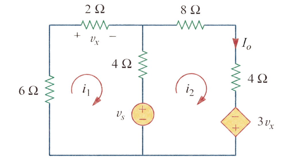
Figure 2 – Circuit diagram for Pb-1

Solution

Figure 3 – Circuit diagram for solving the Pb-1

\small \begin{aligned} &\text{KVL at mesh 1,} \\[2ex] & 6i_1 + 2i_1 + 4(i_1 - i_2) + v_s = 0 \\[2ex] & \Rightarrow 6i_1 + 2i_1 + 4i_1 - 4i_2 = -v_s \\[2ex] & \therefore 12i_1 - 4i_2 = -v_s \quad \text{\text{-} \text{-} \text{-} (i)} \\[3ex] &\text{KVL at mesh 2,} \\[2ex] & -v_s + 4(i_2 - i_1) + 8i_2 + 4i_2 - 3v_x = 0 \\[2ex] & \Rightarrow 4i_2 - 4i_1 + 8i_2 + 4i_2 - 3 \cdot 2i_1 = v_s \\[2ex] & \Rightarrow 4i_2 - 4i_1 + 8i_2 + 4i_2 - 6i_1 = v_s \\[2ex] & \therefore -10i_1 + 16i_2 = v_s \quad \text{\text{-} \text{-} \text{-} (ii)} \\[3ex] &\text{When } v_s = 24 \ V, \\[1ex] & \quad \text{From (i),} \\[1ex] & \quad \quad 12i_1 - 4i_2 = -24 \quad \text{\text{-} \text{-} \text{-} (iii)} \\[1ex] & \quad \text{From (ii),} \\[1ex] & \quad \quad -10i_1 + 16i_2 = 24 \quad \text{\text{-} \text{-} \text{-} (iv)} \\[1ex] & \quad \text{Solving equations (iii) \& (iv),} \\[1ex] & \quad \quad \therefore i_1 = -\frac{36}{19} \ A, \ i_2 = \frac{6}{19} \ A \\[1.5ex] & \quad \quad \therefore I_0 = i_2 = \frac{6}{19} \ A \\[3ex] &\text{When } v_s = 12 \ V, \\[1ex] & \quad \text{From (i),} \\[1ex] & \quad \quad 12i_1 - 4i_2 = -12 \quad \text{\text{-} \text{-} \text{-} (v)} \\[1ex] & \quad \text{From (ii),} \\[1ex] & \quad \quad -10i_1 + 16i_2 = 12 \quad \text{\text{-} \text{-} \text{-} (vi)} \\[1ex] & \quad \text{Solving equations (v) \& (vi),} \\[1ex] & \quad \quad \therefore i_1 = -\frac{18}{19} \ A, \ i_2 = \frac{3}{19} \ A \\[1.5ex] & \quad \quad \therefore I_0 = i_2 = \frac{3}{19} \ A \end{aligned}

Problem 2

Pb-2: For the circuit in Fig. 4, find v_{0} when i_{s} = 30 \ A and i_{s} = 45 \ A .

Figure 4 – Circuit diagram for Pb-2

Solution

Figure 5 – Circuit diagram for solving the Pb-2

\small \begin{aligned} &\text{KCL at node 1,} \\[2ex] & \quad -i_s + \frac{v_1}{4} + \frac{v_1-v_2}{12} = 0 \\[2ex] & \quad \Rightarrow \frac{3v_1+v_1-v_2}{12} = i_s \\[2ex] & \quad \therefore 4v_1 - v_2 = 12i_s \quad \text{\text{-} \text{-} \text{-} (i)} \\[3ex] &\text{KCL at node 2,} \\[2ex] & \quad \frac{v_2-v_1}{12} + \frac{v_2}{8} = 0 \\[2ex] & \quad \Rightarrow \frac{2v_2-2v_1+3v_2}{24} = 0 \\[2ex] & \quad \therefore -2v_1 + 5v_2 = 0 \quad \text{\text{-} \text{-} \text{-} (ii)} \\[3ex] &\text{When } i_s = 30 \ A, \\[1ex] & \quad \text{From (i),} \\[1ex] & \quad \quad 4v_1 - v_2 = 12 \times 30 \\[1ex] & \quad \quad \therefore 4v_1 - v_2 = 360 \quad \text{\text{-} \text{-} \text{-} (iii)} \\[1ex] & \quad \text{Solving equations (ii) \& (iii),} \\[1ex] & \quad \quad \therefore v_1 = 100 \ V, \ v_2 = 40 \ V \\[1.5ex] & \quad \quad \therefore v_0 = v_2 = 40 \ V \\[3ex] &\text{When } i_s = 45 \ A, \\[1ex] & \quad \text{From (i),} \\[1ex] & \quad \quad 4v_1 - v_2 = 12 \times 45 \\[1ex] & \quad \quad \therefore 4v_1 - v_2 = 540 \quad \text{\text{-} \text{-} \text{-} (iv)} \\[1ex] & \quad \text{Solving equations (ii) \& (iv),} \\[1ex] & \quad \quad \therefore v_1 = 150 \ V, \ v_2 = 60 \ V \\[1.5ex] & \quad \quad \therefore v_0 = v_2 = 60 \ V \end{aligned}

Problem 3

Pb-3: Assume I_{0} = 1 \ A and use linearity to find the actual value of I_{0} in the circuit of Fig. 6.

Figure 6 – Circuit diagram for Pb-3

Solution

Figure 7 – Circuit diagram for solving the Pb-3

\small \begin{aligned} &\text{Assuming } I_0 = 1 \ A, \\[2ex] & \quad \therefore V_1 = (3 + 5)I_0 = 8 \times 1 = 8 \ V \\[2ex] & \quad \& \ I_1 = \frac{V_1}{4} = \frac{8}{4} = 2 \ A \\[2ex] & \quad \text{KCL at node 1,} \\[2ex] & \quad I_0 + I_1 - I_2 = 0 \Rightarrow 1 + 2 - I_2 = 0 \\[2ex] & \quad \therefore I_2 = 3 \ A \\[3ex] & \quad \text{Now,} \\[2ex] & \quad \quad I_2 = \frac{V_2 - V_1}{2} \\[2.5ex] & \quad \quad \Rightarrow 3 = \frac{V_2 - 8}{2} \\[2ex] & \quad \quad \therefore V_2 = 14 \ V \\[3ex] & \quad \text{Again,} \\[2ex] & \quad \quad I_3 = \frac{V_2}{7} = \frac{14}{7} = 2 \ A \\[3ex] & \quad \text{KCL at node 2,} \\[2ex] & \quad I_2 + I_3 - I_4 = 0 \Rightarrow 3 + 2 - I_4 = 0 \\[2ex] & \quad \therefore I_4 = 5 \ A \\[2ex] &\therefore I_s = I_4 = 5 \ A \\[3ex] &\text{This shows that assuming } I_0 = 1 \ A \text{ gives } \\[0.5ex] & I_s = 5 \ A. \text{ Therefore, the actual source current, } \\[0.5ex] & I_s = 15 \ A \text{ will give } I_0 = 3 \ A \text{ as the actual value.} \end{aligned}

Problem 4

Pb-4: Assume that V_{0} = 1 \ V and use linearity to calculate the actual value of V_{0} in the circuit of Fig. 8.

Figure 8 – Circuit diagram for Pb-4

Solution

Figure 9 – Circuit diagram for solving the Pb-4

\small \begin{aligned} &\text{Assuming } V_0 = 1 \ V, \\[2ex] & \quad \therefore I_1 = \frac{V_0}{8} = \frac{1}{8} \ A \\[3ex] & \quad \text{Now,} \\[2ex] & \quad I_1 = \frac{V_1 - V_0}{12} \\[2ex] & \quad \Rightarrow \frac{1}{8} = \frac{V_1 - 1}{12} \\[2ex] & \quad \therefore V_1 = 2.5 \ V \\[2ex] &\therefore V_s = V_1 = 2.5 \ V \\[3ex] &\text{This shows that assuming } V_0 = 1 \ V \text{ gives } \\[0.5ex] & V_s = 2.5 \ V. \text{ Therefore, the actual source } \\[0.5ex] & \text{ voltage, } V_s = 40 \ V \text{ will give } V_0 = 16 \ V \\[0.5ex] & \text{ as the actual value. } \end{aligned}

SuperPosition Theorem

The superposition principle states that the voltages across (or currents through)  an element in a linear circuit is the algebraic sum of the voltages across (or currents through) that element due to each independent source acting alone.

It helps us to analyze a linear circuit with more than one independent source by calculating the contribution of each independent source separately.

Fundamental Rules of Superposition

To apply the superposition principle correctly, we must keep these two rules in mind

1. Isolate Independent Sources

Let’s suppose that we need to find v_{0} using SuperPosition Principle in the circuit of Fig. 10.

Figure 10 – Circuit diagram to apply superposition principle

• Voltage source will be short circuited.

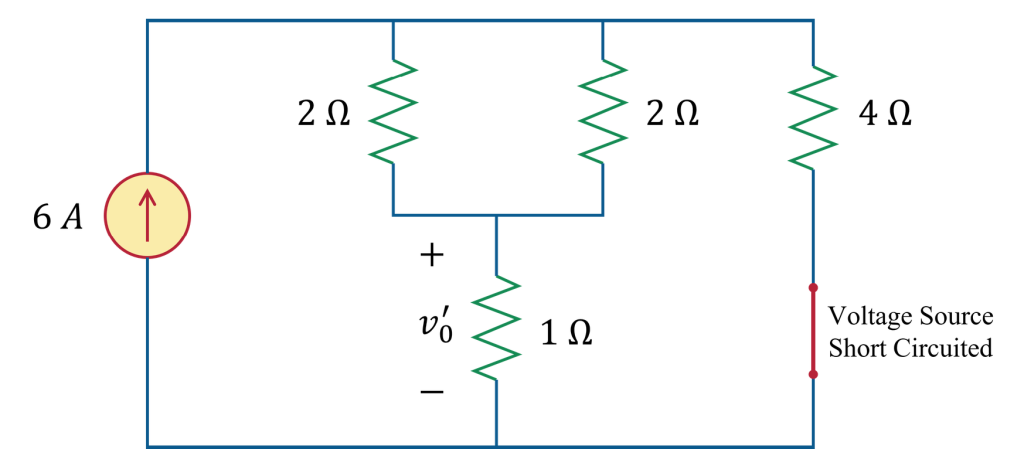
Figure 11 – Short circuited voltage source for superposition principle

• Current source will be open circuited.

Figure 12 – Open circuited current source for superposition principle

2. Leave Dependent Sources Intact

Let’s suppose that we need to find i_{0} and v_{0} using SuperPosition Principle in the circuit of Fig. 13.

Figure 13 – Circuit diagram to apply superposition principle (with dependent source)

• Dependent source won’t be replaced.

Figure 14 – Short circuited voltage source for superposition principle (with dependent source)

Figure 15 – Open circuited current source for superposition principle (with dependent source)

Steps to Apply Superposition Theorem

Figure 16 – Circuit diagram to apply superposition theorem

we need to find i_{0} and v_{0} using SuperPosition Theorem in the circuit of Fig. 16.

1. Activate One Source at a Time

Figure 17 – Activating current source

Figure 18 – Activating voltage source

2. Solve for All Independent Sources

\small \begin{aligned} &\text{Let,} \\[1ex] & \quad v_0 = v_0' + v_0'' \\[2ex] &\text{Where,} \\[1ex] & \quad v_0' = \text{contribution due to } 6 \ A \text{ current source} \\[1ex] & \quad v_0'' = \text{contribution due to } 30 \ V \text{ voltage source} \end{aligned}

Figure 19 – Solving for current source

\small \begin{aligned} &\text{KCL at node 1,} \\[2ex] & -6 + \frac{v_1}{40} + \frac{v_1-v_2}{10} = 0 \\[2ex] & \Rightarrow \frac{-240+v_1+4v_1-4v_2}{40} = 0 \\[2ex] & \therefore 5v_1 - 4v_2 = 240 \quad \text{\text{-} \text{-} \text{-} (i)} \\[3ex] &\text{KCL at node 2,} \\[2ex] & \frac{v_2}{20} - 4i_0' + \frac{v_2-v_1}{10} = 0 \\[2ex] & \Rightarrow \frac{v_2}{20} - 4 \cdot \frac{v_1-v_2}{10} + \frac{v_2-v_1}{10} = 0 \\[2.5ex] & \Rightarrow \frac{v_2-8v_1+8v_2+2v_2-2v_1}{20} = 0 \\[2ex] & \therefore -10v_1 + 11v_2 = 0 \quad \text{\text{-} \text{-} \text{-} (ii)} \\[3ex] &\text{Solving equations (i) and (ii),} \\[2ex] & \therefore v_1 = 176 \ V, \ v_2 = 160 \ V \\[2ex] & \therefore v_0' = v_1 - v_2 = 176 - 160 = 16 \ V \end{aligned}

Figure 20 – Solving for voltage source

\small \begin{aligned} &\text{KCL at node 3,} \\[2ex] & \frac{v_3}{40} + \frac{v_3-v_4}{10} = 0 \\[2ex] & \Rightarrow \frac{v_3+4v_3-4v_4}{40} = 0 \\[2ex] & \therefore 5v_3 - 4v_4 = 0 \quad \text{---(iii)} \\[3ex] &\text{KCL at node 4,} \\[2ex] & \frac{v_4-(-30)}{20} - 4i_0'' + \frac{v_4-v_3}{10} = 0 \\[2ex] & \Rightarrow \frac{v_4+30}{20} - 4 \cdot \frac{v_3-v_4}{10} + \frac{v_4-v_3}{10} = 0 \\[2.5ex] & \Rightarrow \frac{v_4+30-8v_3+8v_4+2v_4-2v_3}{20} = 0 \\[2ex] & \therefore -10v_3 + 11v_4 = -30 \quad \text{---(iv)} \\[3ex] &\text{Solving equations (iii) and (iv),} \\[2ex] & \therefore v_3 = -8 \ V, \ v_4 = -10 \ V \\[2ex] & \therefore v_0'' = v_3 - v_4 = -8 - (-10) = 2 \ V \end{aligned}

3. Algebraic Summation

\small \begin{aligned} &\text{We get,} \\[2ex] & \quad v_0' = 16 \ V \\[2ex] & \quad v_0'' = 2 \ V \\[3ex] &\text{Now,} \\[2ex] & \quad v_0 = v_0' + v_0'' = 16 + 2 \\[2ex] & \quad \therefore v_0 = 18 \ V \\[3ex] &\text{Again,} \\[2ex] & \quad i_0 = \frac{v_0}{10} = \frac{18}{10} \\[3ex] & \quad \therefore i_0 = 1.8 \ A \end{aligned}

Solved Problems on Superposition Theorem

Problem 5

Pb-5: Use the superposition theorem to find v in the circuit of Fig. 21.

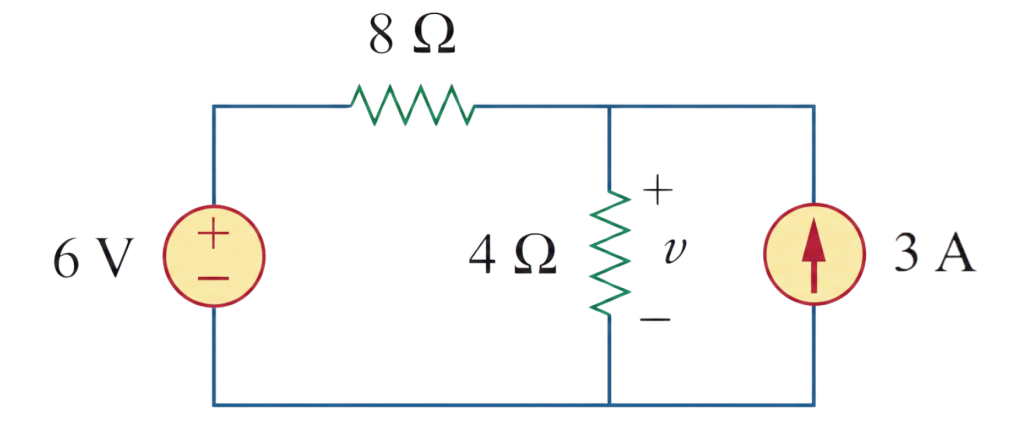
Figure 21 – Circuit diagram for Pb-5

Solution:

\small \begin{aligned} &\text{Let,} \\[1ex] & \quad v = v_1 + v_2 \\[2ex] &\text{Where,} \\[1ex] & \quad v_1 = \text{contribution due to } 6 \ V \text{ voltage source} \\[1ex] & \quad v_2 = \text{contribution due to } 3 \ A \text{ current source} \end{aligned}

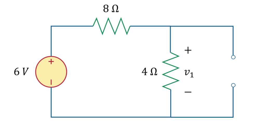
Figure 22 – Circuit diagram for solving the Pb-5 (activating 6 \ V voltage source)

\small \begin{aligned} &\text{Using voltage division rule,} \\[2ex] & v_1 = \frac{4}{4+8} \times 6 \\[2ex] & \therefore v_1 = 2 \ V \end{aligned}

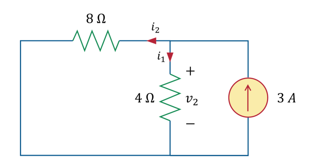
Figure 23 – Circuit diagram for solving the Pb-5 (activating 3 \ A current source)

\small \begin{aligned} &\text{Using current division rule,} \\[2.5ex] & i_1 = \frac{8||4}{4} \times 3 \\[2.5ex] & \Rightarrow i_1 = \frac{(8^{-1} + 4^{-1})^{-1}}{4} \times 3 \\[2.5ex] & \therefore i_1 = 2 \ A \\[2ex] & \therefore v_2 = 4i_1 = 4 \times 2 = 8 \ V \end{aligned}

\small \begin{aligned} &\text{We get,} \\[2ex] & \quad v_1 = 2 \ V \\[2ex] & \quad v_2 = 8 \ V \\[3ex] &\text{Now,} \\[2ex] & \quad v = v_1 + v_2 = 2 + 8 \\[2ex] & \quad \therefore v = 10 \ V \end{aligned}

Problem 6

Pb-6: Using the superposition theorem, find v_0 in the circuit of Fig. 24.

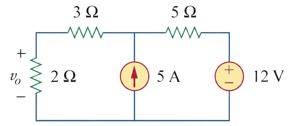
Figure 24 – Circuit diagram for Pb-6

Solution:

\small \begin{aligned} &\text{Let,} \\[1ex] & \quad v_0 = v_1 + v_2 \\[2ex] &\text{Where,} \\[1ex] & \quad v_1 = \text{contribution due to } 5 \ A \text{ current source} \\[1ex] & \quad v_2 = \text{contribution due to } 12 \ V \text{ voltage source} \end{aligned}

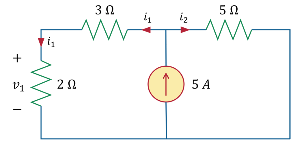
Figure 25 – Circuit diagram for solving the Pb-6 (activating 5 \ A current source)

\small \begin{aligned} &\text{Using current division rule,} \\[2.5ex] & i_1 = \frac{((3+2)||5)}{(3+2)} \times 5 = \frac{((3+2)^{-1}+5^{-1})^{-1}}{(3+2)} \times 5 \\[2.5ex] & \therefore i_1 = 2.5 \ A \\[2.5ex] & \therefore v_1 = 2i_1 = 2 \times 2.5 = 5 \ V \end{aligned}

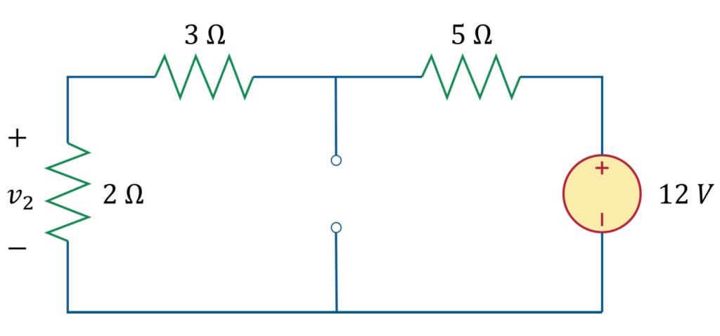
Figure 26 – Circuit diagram for solving the Pb-6 (activating 12 \ V voltage source)

\small \begin{aligned} &\text{Using voltage division rule,} \\[2ex] & v_2 = \frac{2}{2+3+5} \times 12 \\[2ex] & \therefore v_2 = 2.4 \ V \end{aligned}

\small \begin{aligned} &\text{We get,} \\[2ex] & \quad v_1 = 5 \ V \\[2ex] & \quad v_2 = 2.4 \ V \\[3ex] &\text{Now,} \\[2ex] & \quad v_0 = v_1 + v_2 = 5 + 2.4 \\[2ex] & \quad \therefore v_0 = 7.4 \ V \end{aligned}

Problem 7

Pb-7: Find i_0 in the circuit of Fig. 27 using superposition.

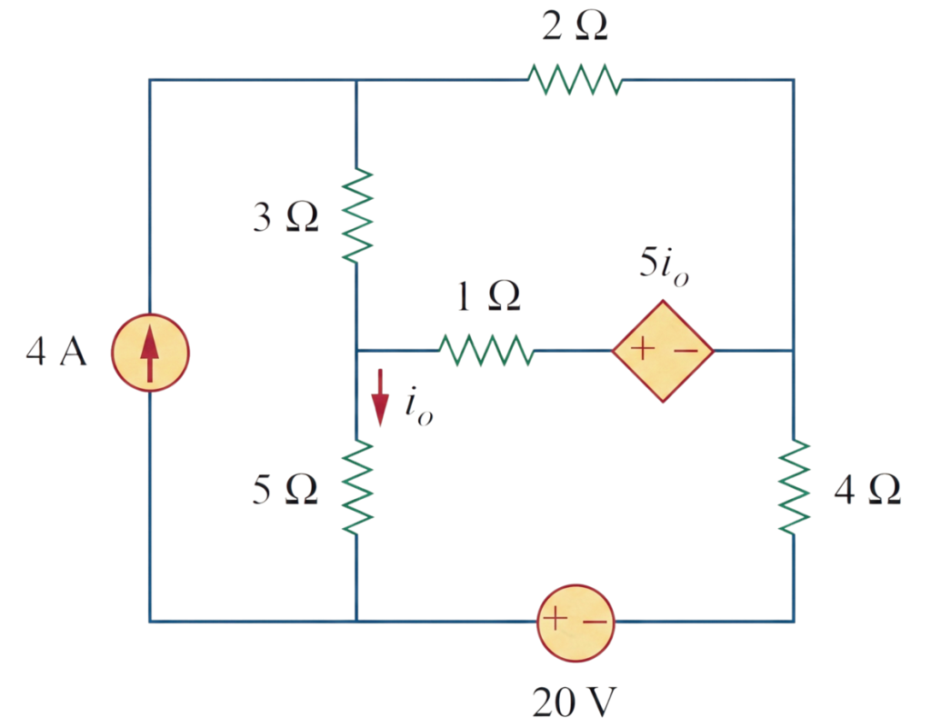
Figure 27 – Circuit diagram for Pb-7

Solution:

\small \begin{aligned} &\text{Let,} \\[1ex] & \quad i_0 = i_0' + i_0'' \\[2ex] &\text{Where,} \\[1ex] & \quad i_0' = \text{contribution due to } 4 \ A \text{ current source} \\[1ex] & \quad i_0'' = \text{contribution due to } 20 \ V \text{ voltage source} \end{aligned}

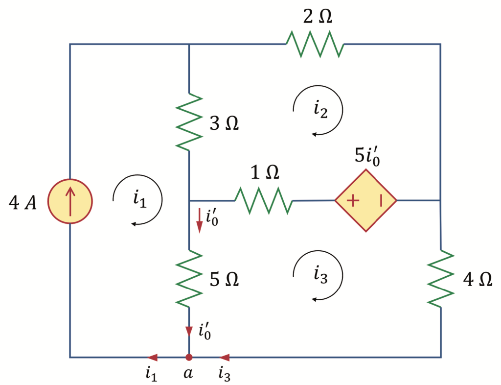
Figure 28 – Circuit diagram for solving the Pb-7 (activating 4 \ A current source)

\small \begin{aligned} &\text{KCL at node a,} \\[2ex] & i_1 - i_0' - i_3 = 0 \\[2ex] & \therefore i_0' = i_1 - i_3 \\[2ex] & \text{For mesh 1,} \\[2ex] & \therefore i_1 = 4 \quad \text{\text{-} \text{-} \text{-} (i)} \\[2ex] & \text{KVL at mesh 2,} \\[2ex] & 3(i_2 - i_1) + 2i_2 - 5i_0' + (i_2 - i_3) = 0 \\[2ex] & \Rightarrow 3(i_2 - i_1) + 2i_2 - 5(i_1 - i_3) + (i_2 - i_3) = 0 \\[2ex] & \Rightarrow 3i_2 - 3i_1 + 2i_2 - 5i_1 + 5i_3 + i_2 - i_3 = 0 \\[2ex] & \therefore -8i_1 + 6i_2 + 4i_3 = 0 \quad \text{\text{-} \text{-} \text{-} (ii)} \\[2ex] & \text{KVL at mesh 3,} \\ &5(i_3 - i_1) + (i_3 - i_2) + 5i_0' + 4i_3 = 0 \\[2ex] & \Rightarrow 5(i_3 - i_1) + (i_3 - i_2) + 5(i_1 - i_3) + 4i_3 = 0 \\[2ex] & \Rightarrow 5i_3 - 5i_1 + i_3 - i_2 + 5i_1 - 5i_3 + 4i_3 = 0 \\[2ex] & \therefore -i_2 + 5i_3 = 0 \quad \text{\text{-} \text{-} \text{-} (iii)} \\[2ex] & \text{Solving equations (i), (ii) and (iii),} \\[2ex] & \therefore i_1 = 4 \ A, \ i_2 = 4.71 \ A, \ i_3 = 0.94 \ A \\[2ex] & \therefore i_0' = i_1 - i_3 = 4 - 0.94 = 3.06 \ A \end{aligned}

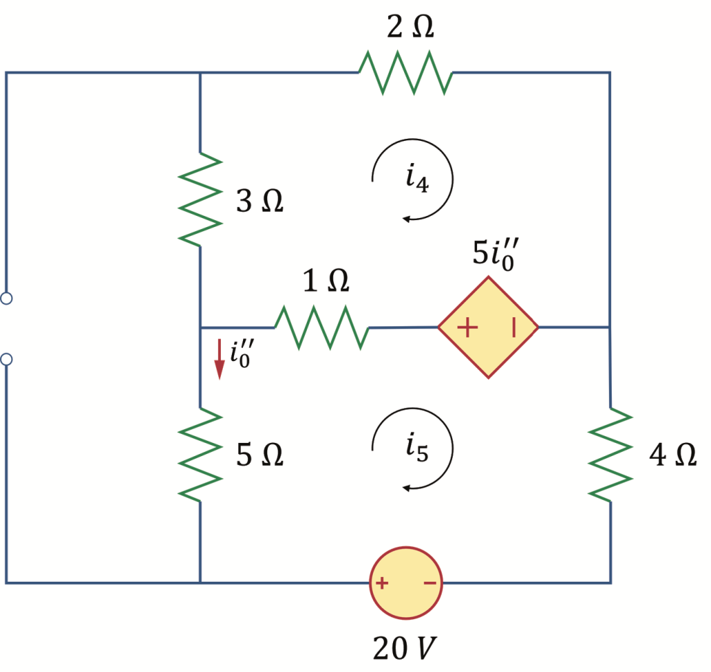
Figure 29 – Circuit diagram for solving the Pb-7 (activating 20 \ V voltage source)

  \small \begin{aligned} &\text{KVL at mesh 4,} \\[2ex] & 3i_4 + 2i_4 - 5i_0'' + (i_4 - i_5) = 0 \\[2ex] & \Rightarrow 3i_4 + 2i_4 - 5 \cdot (-i_5) + (i_4 - i_5) = 0 \\[2ex] & \Rightarrow 3i_4 + 2i_4 + 5i_5 + i_4 - i_5 = 0 \\[2ex] & \therefore 6i_4 + 4i_5 = 0 \quad \text{\text{-} \text{-} \text{-} (iv)} \\[2ex] & \text{KVL at mesh 5,} \\[2ex] & 5i_5 + (i_5 - i_4) + 5i_0'' + 4i_5 - 20 = 0 \\[2ex] & \Rightarrow 5i_5 + (i_5 - i_4) + 5 \cdot (-i_5) + 4i_5 = 20 \\[2ex] & \Rightarrow 5i_5 + i_5 - i_4 - 5i_5 + 4i_5 = 20 \\[2ex] & \therefore -i_4 + 5i_5 = 20 \quad \text{\text{-} \text{-} \text{-} (v)} \\[2ex] & \text{Solving equations (iv) and (v),} \\[2ex] & \therefore i_4 = -2.35 \ A, \ i_5 = 3.53 \ A \\[2ex] & \therefore i_0'' = -i_5 = -3.53 \ A \end{aligned}

\small \begin{aligned} &\text{We get,} \\[2ex] & \quad i_0' = 3.06 \ A \\[2ex] & \quad i_0'' = -3.53 \ A \\[3ex] &\text{Now,} \\[2ex] & \quad i_0 = i_0' + i_o'' = 3.06 + (-3.53) \\[2ex] & \quad \therefore i_0 = -0.47 \ A \end{aligned}

Problem 8

Pb-8: Use superposition to find v_x in the circuit of Fig. 30.

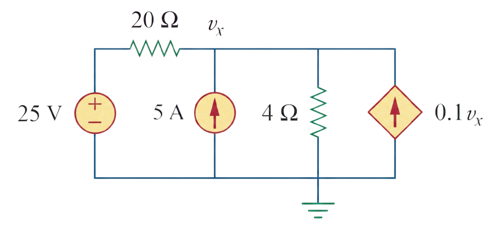
Figure 30 – Circuit diagram for Pb-8

Solution:

\small \begin{aligned} &\text{Let,} \\[1ex] & \quad v_x = v_1 + v_2 \\[2ex] &\text{Where,} \\[1ex] & \quad v_1 = \text{contribution due to } 25 \ V \text{ voltage source} \\[1ex] & \quad v_2 = \text{contribution due to } 5 \ A \text{ current source} \end{aligned}

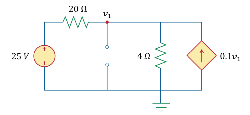
Figure 31 – Circuit diagram for solving the Pb-8 (activating 25 \ V voltage source)

\small \begin{aligned} &\text{KCL at node 1,} \\[2ex] & \frac{v_1 - 25}{20} + \frac{v_1}{4} - 0.1v_1 = 0 \\[2ex] & \therefore v_1 = 6.25 \ V \end{aligned}

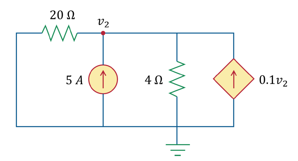
Figure 32 – Circuit diagram for solving the Pb-8 (activating 5 \ A current source)

\small \begin{aligned} &\text{KCL at node 2,} \\[2ex] & \frac{v_2}{20} - 5 + \frac{v_2}{4} - 0.1v_2 = 0 \\[2ex] & \therefore v_2 = 25 \ V \end{aligned}

\small \begin{aligned} &\text{We get,} \\[2ex] & \quad v_1 = 6.25 \ V \\[2ex] & \quad v_2 = 25 \ V \\[3ex] &\text{Now,} \\[2ex] & \quad v_x = v_1 + v_2 = 6.25 + 25 \\[2ex] & \quad \therefore v_x = 31.25 \ V \end{aligned}

Problem 9

Pb-9: For the circuit of Fig. 33, use the superposition principle to find i .

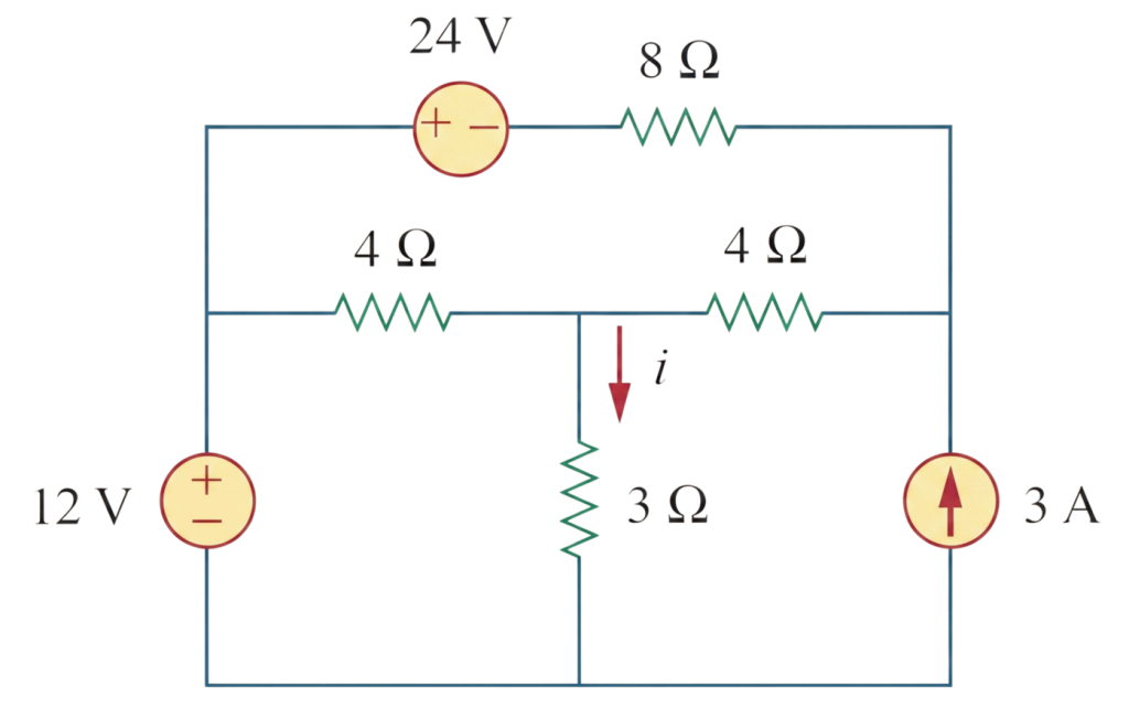
Figure 33 – Circuit diagram for Pb-9

Solution:

\small \begin{aligned} &\text{Let,} \\[1ex] & \quad i = i_1 + i_2 + i_3 \\[2ex] &\text{Where,} \\[1ex] & \quad i_1 = \text{contribution due to } 12 \ V \text{ voltage source} \\[1ex] & \quad i_2 = \text{contribution due to } 24 \ V \text{ voltage source} \\[1ex] & \quad i_3 = \text{contribution due to } 3 \ A \text{ current source} \end{aligned}

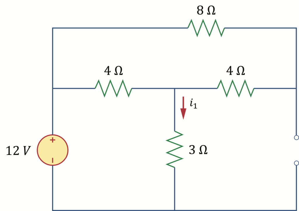
Figure 34 – Circuit diagram for solving the Pb-9 (activating 12 \ V voltage source)

Simplifying the circuit in Fig. 34,

Figure 35 – Circuit diagram for solving the Pb-9 (for finding i_1 )

\small \begin{aligned} &\text{Using Ohm's Law,} \\[2ex] &\quad i_1 = \frac{12}{3+3} \\[2ex] &\quad \therefore i_1 = 2 \ A \end{aligned}

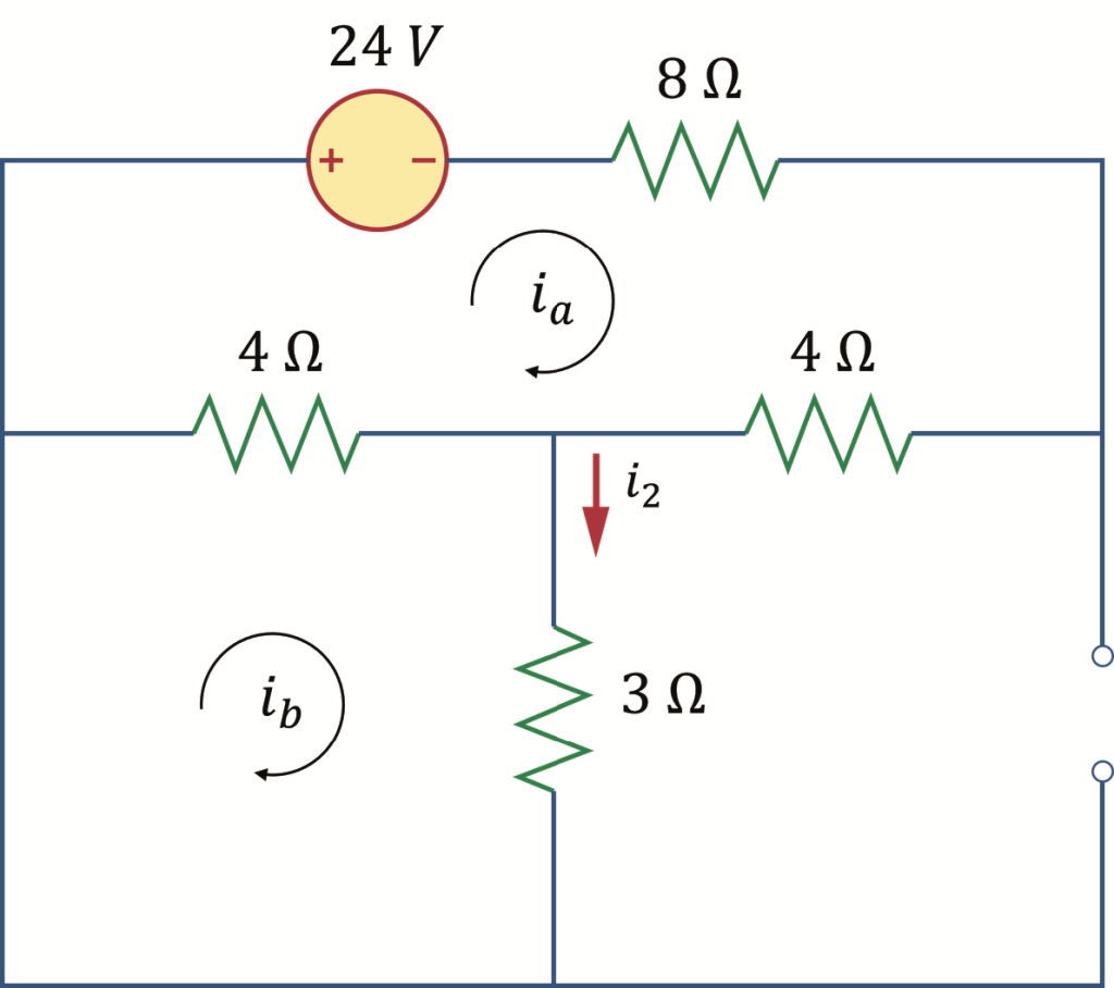
Figure 36 – Circuit diagram for solving the Pb-9 (activating 24 \ V voltage source)

\small \begin{aligned} &\text{KVL at mesh a,} \\[2ex] & 4(i_a - i_b) + 24 + 8i_a + 4i_a = 0 \\[2ex] & \Rightarrow 4i_a - 4i_b + 8i_a + 4i_a = -24 \\[2ex] & \therefore 16i_a - 4i_b = -24 \quad \text{\text{-} \text{-} \text{-} (i)} \\[2ex] & \text{KVL at mesh b,} \\[2ex] & 4(i_b - i_a) + 3i_b = 0 \\[2ex] & \Rightarrow 4i_b - 4i_a + 3i_b = 0 \\[2ex] & \therefore -4i_a + 7i_b = 0 \quad \text{\text{-} \text{-} \text{-} (ii)} \\[2ex] & \text{Solving equations (i) and (ii),} \\[2ex] & \therefore i_a = -1.75 \ A, \ i_b = -1 \ A \\[2ex] & \therefore i_2 = i_b = -1 \ A \end{aligned}

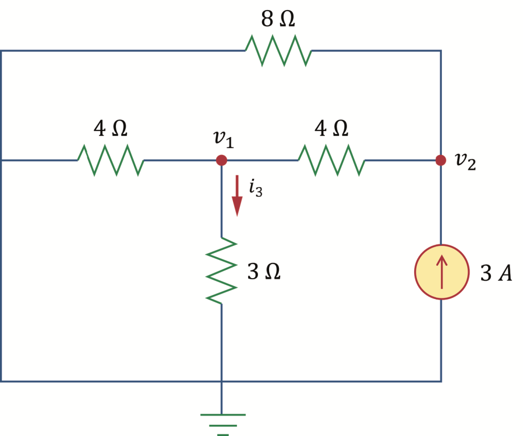
Figure 37 – Circuit diagram for solving the Pb-9 (activating 3 \ A current source)

\small \begin{aligned} &\text{KCL at node 1,}\\[2ex] & \frac{v_1}{4} + \frac{v_1}{3} + \frac{v_1 - v_2}{4} = 0 \\[2ex] & \Rightarrow \frac{3v_1 + 4v_1 + 3v_1 - 3v_2}{12} = 0 \\[2ex] & \therefore 10v_1 - 3v_2 = 0 \quad \text{\text{-} \text{-} \text{-} (iii)} \\[2ex] & \text{KCL at node 2,} \\[2ex] & -3 + \frac{v_2 - v_1}{4} + \frac{v_2}{8} = 0 \\[2ex] & \Rightarrow \frac{-24 + 2v_2 - 2v_1 + v_2}{8} = 0 \\[2ex] & \therefore -2v_1 + 3v_2 = 24 \quad \text{\text{-} \text{-} \text{-} (iv)} \\[2ex] & \text{Solving equations (iii) and (iv),} \\[2ex] & \therefore v_1 = 3 \ V, \ v_2 = 10 \ V \\[2ex] & \therefore i_3 = \frac{v_1}{3} = \frac{3}{3} = 1 \ A \end{aligned}

\small \begin{aligned} &\text{We get,} \\[2ex] & \quad i_1 = 2 \ A \\[2ex] & \quad i_2 = -1 \ A \\[2ex] & \quad i_3 = 1 \ A \\[3ex] &\text{Now,} \\[2ex] & \quad i = i_1 + i_2 + i_3 = 2 - 1 + 1 \\[2ex] & \quad \therefore i = 2 \ A \end{aligned}

Problem 10

Pb-10: Find I in the circuit of Fig. 38, using superposition principle.

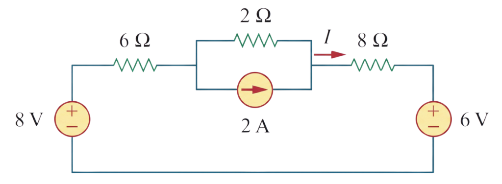
Figure 38 – Circuit diagram for Pb-10

Solution:

\small \begin{aligned} &\text{Let,} \\[1ex] & \quad I = I_1 + I_2 + I_3 \\[2ex] &\text{Where,} \\[1ex] & \quad I_1 = \text{contribution due to } 8 \ V \text{ voltage source} \\[1ex] & \quad I_2 = \text{contribution due to } 2 \ A \text{ current source} \\[1ex] & \quad I_3 = \text{contribution due to } 6 \ V \text{ voltage source} \end{aligned}

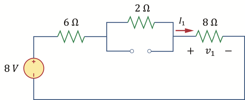
Figure 39 – Circuit diagram for solving the Pb-10 (activating 8 \ V voltage source)

\small \begin{aligned} &\text{Using voltage division rule,} \\[2ex] & v_1 = \frac{8}{6+2+8} \times 8 \\[2ex] & \therefore v_1 = 4 \ V \\[2ex] & \therefore I_1 = \frac{v_1}{8} = \frac{4}{8} = 0.5 \ A \end{aligned}

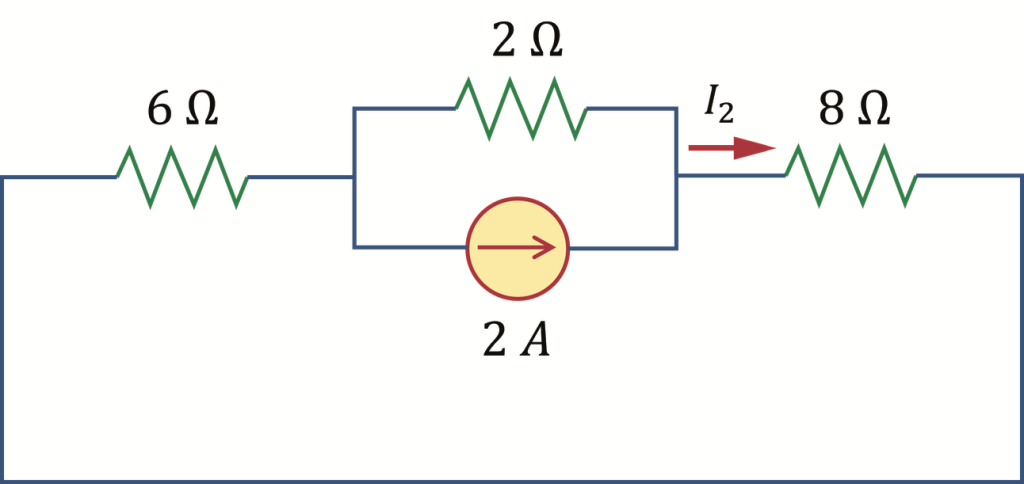
Figure 40 – Circuit diagram for solving the Pb-10 (activating 2 \ A current source)

\small \begin{aligned} &\text{Using current division rule,} \\[2.5ex] & I_2 = \frac{((6+8)||2)}{(6+8)} \times 2 \\[2.5ex] & \Rightarrow I_2 = \frac{((6+8)^{-1}+2^{-1})^{-1}}{(6+8)} \times 2 \\[2.5ex] & \therefore I_2 = 0.25 \ A \end{aligned}

Figure 41 – Circuit diagram for solving the Pb-10 (activating 6 \ V voltage source)

\small \begin{aligned} &\text{Using voltage division rule,} \\[2ex] & v_3 = -\frac{8}{6+2+8} \times 6 \\[2ex] & \therefore v_3 = -3 \ V \\[2ex] & \therefore I_3 = \frac{v_3}{8} = \frac{-3}{8} = -0.375 \ A \end{aligned}

\small \begin{aligned} &\text{We get,} \\[2ex] & \quad I_1 = 0.5 \ A \\[2ex] & \quad I_2 = 0.25 \ A \\[2ex] & \quad I_3 = -0.375 \ A \\[3ex] &\text{Now,} \\[2ex] & \quad I = I_1 + I_2 + I_3 = 0.5 + 0.25 - 0.375 \\[2ex] & \quad \therefore I = 0.375 \ A \end{aligned}

Source Transformation

A source transformation is the process of replacing a voltage source v_s in series with a resistor R by a current source i_s in parallel with a resistor R or vice versa.

Source Transformation is a powerful tool that allows circuit manipulations to ease circuit analysis.

Figure 42 – Transformation of independent sources

Figure 43 – Transformation of dependent sources

Source transformation requires that:

\small v_s = i_s R \qquad \text{or} \qquad i_s = \frac{v_s}{R}

Important rules for Source Transformation

To apply the source transformation correctly, we must keep these two rules in mind

1. Align Source Polarity and Direction

Figure 44 – Transforming voltage source to current source

\small \begin{aligned} &\text{From Ohm's Law,} \\[2ex] &\quad i = \frac{v}{R} = \frac{9}{2} = 4.5 \ A \end{aligned}

Figure 45 – Transforming current source to voltage source

\small \begin{aligned} &\text{From Ohm's Law,} \\[2ex] &\quad v = iR = 4.5 \times (2||4) = 4.5 \times (2^{-1} + 4^{-1})^{-1} \\[2ex] &\quad \phantom{v} = 4.5 \times 1.33 = 5.985 \ V \end{aligned}

2. Protect the Target Variable

Let’s suppose that we need to find v_0 in the circuit of Fig. 46 using source transformation.

Figure 46 – Circuit diagram to apply source transformation

As it is asked to find the voltage drop between the 1 \ k \Omega resistor, so we won’t transform this resistor.

Using source transformation in Fig. 46,

Figure 47 – Converting voltage source to current source

Using source transformation in Fig. 47,

Figure 48 – Converting current source to voltage source

Leave the 1 \ k \Omega resistor untouched because we are calculating the voltage drop across it.

Steps to Apply Source Transformation

Figure 49 – Circuit diagram for applying source transformation

we need to find v_0 using Source Transformation in the circuit of Fig. 49.

1. Identify the Target Source

Figure 50 – Identifying the target source

2. Convert the Source Value

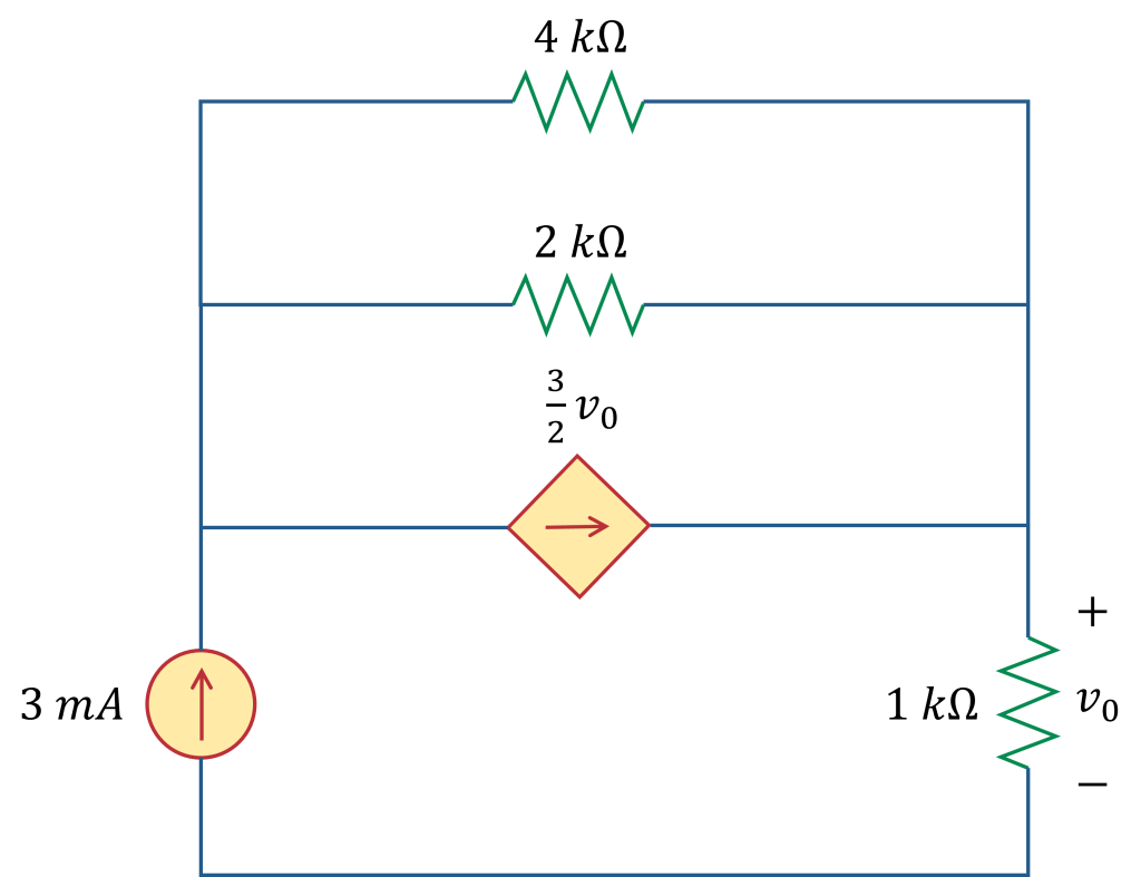
Figure 51 – Converting the source value

3. Repeat Till Simplified

Figure 52 – Repeating the source transformation

4. Calculate the Final Answer

Figure 53 – Calculating the final answer

\small \begin{aligned} &\text{From Fig. 4.53,} \\ &\qquad\qquad i_0 = 3 \ mA \\[2ex] &\text{Now,} \\[1ex] &\quad v_0 = 1i_0 \\ &\quad \phantom{v_0} = 1 \times 3 \\ &\quad \phantom{v_0} = 3 \ V \end{aligned}

Solved Problems on Source Transformation

Problem 11

Pb-11: Use source transformation to find v_0 in the circuit of Fig. 54.

Figure 54 – Circuit diagram for Pb-11

Solution:

Using source transformation in Fig. 54,

Figure 55 – Circuit diagram for solving the Pb-11 (transforming left current source and right voltage source of Fig. 54)

Using source transformation in Fig. 55,

Figure 56 – Circuit diagram for solving the Pb-11 (transforming left voltage source of Fig. 55)

Using source transformation in Fig. 56,

Figure 57 – Circuit diagram for solving the Pb-11 (final transformation for finding v_0 )

\small \begin{aligned} &\text{Using current divider rule in Fig. 4.57,} \\[2.5ex] & i_0 = \frac{2||8}{8} \times 2 = \frac{(2^{-1}+8^{-1})^{-1}}{8} \times 2 \\[2.5ex] & \therefore i_0 = 0.4 \ A \\[2ex] &\text{Now,} \\[2ex] & v_0 = 8i_0 = 8 \times 0.4 \\[2ex] & \therefore v_0 = 3.2 \ V \end{aligned}

Problem 12

Pb-12: Find i_0 in the circuit of Fig. 58 using source transformation.

Figure 58 – Circuit diagram for Pb-12

Solution:

Using source transformation in Fig. 58,

Figure 59 – Circuit diagram for solving the Pb-12 (transforming source for finding i_0 )

\small \begin{aligned} &\text{KCL at node 0,} \\[2ex] & \frac{v_0 - 5 - 10}{2} + \frac{v_0 - 15}{5} + \frac{v_0}{7} = 0 \\[2.5ex] & \Rightarrow \frac{v_0 - 15}{2} + \frac{v_0 - 15}{5} + \frac{v_0}{7} = 0 \\[2.5ex] & \Rightarrow \frac{35v_0 - 525 + 14v_0 - 210 + 10v_0}{70} = 0 \\[2.5ex] & \Rightarrow 59v_0 - 735 = 0 \\[2ex] & \Rightarrow v_0 = \frac{735}{59} \\[2ex] & \therefore v_0 = 12.46 \ V \\[2ex] &\text{Now,} \\[2ex] & i_0 = \frac{v_0}{7} = \frac{12.46}{7} \\[2.5ex] & \therefore i_0 = 1.78 \ A \end{aligned}

Problem 13

Pb-13: Find v_x in Fig. 60 using source transformation.

Figure 60 – Circuit diagram for Pb-13

Solution:

Using source transformation in Fig. 60,

Figure 61 – Circuit diagram for solving the Pb-13 (transforming left voltage source and upper current source of Fig. 60)

Using source transformation in Fig. 61,

Figure 62 – Circuit diagram for solving the Pb-13 (final transformation for finding v_x )

\small \begin{aligned} &\text{KVL at loop 1,} \\[2ex] &-3 + 1i_1 + 4i_1 + v_x + 18 = 0 \\[2ex] & \therefore 5i_1 + v_x = -15 \quad \text{\text{-} \text{-} \text{-} (i)} \\[2ex] &\text{KVL to the loop containing } 3 \ V \text{ voltage source,} \\ &1 \ \Omega \text{ resistor and } v_x \text{ yields,} \\[2ex] &-3 + 1i_1 + v_x = 0 \\[2ex] & \therefore i_1 + v_x = 3 \quad \text{\text{-} \text{-} \text{-} (ii)} \\[2ex] &\text{Solving equations (i) and (ii),} \\[2ex] & \therefore i_1 = -4.5 \ A, \ v_x = 7.5 \ A \\[2ex] &\text{Now,} \\[2ex] & v_x = 7.5 \ A \\[2ex] & \therefore v_x = 7.5 \ A \end{aligned}

Problem 14

Pb-14: Use source transformation to find i_x in the circuit shown in Fig. 63.

Figure 63 – Circuit diagram for Pb-14

Solution:

Using source transformation in Fig. 63,

Figure 64 – Circuit diagram for solving the Pb-14 (transforming source for finding i_x )

\small \begin{aligned} &\text{KCL at node } x, \\[2ex] & -(24 \times 10^{-3}) + \frac{v_x}{10} + \frac{v_x}{5} + \frac{2i_x}{5} = 0 \\[2.5ex] & \Rightarrow -(24 \times 10^{-3}) + \frac{v_x}{10} + \frac{v_x}{5} + \frac{2 \cdot \frac{v_x}{10}}{5} = 0 \\[2.5ex] & \Rightarrow -(24 \times 10^{-3}) + \frac{v_x}{10} + \frac{v_x}{5} + \frac{2v_x}{50} = 0 \\[2.5ex] & \therefore v_x = 0.0706 \ V \\[2ex] &\text{Now,} \\[2ex] & i_x = \frac{v_x}{10} = \frac{0.0706}{10} \\[2ex] & \therefore i_x = 7.06 \times 10^{-3} \ A = 7.06 \ mA \end{aligned}

Thevenin’s Theorem

Thevenin’s theorem states that a linear two-terminal circuit can be replaced by an equivalent circuit consisting of a voltage source V_{Th} in series with a resistor R_{Th} , where V_{Th} is the open-circuit voltage at the terminals and R_{Th} is the input or equivalent resistance at the terminals when the independent sources are turned off.

Thevenin’s theorem is a powerful tool that replaces fixed circuit networks with a simple equivalent circuit to ease the analysis of variable loads.

(a)

(b)

Figure 65 – Replacing a linear two-terminal circuit by its Thevenin equivalent : (a) original circuit , (b) the Thevenin equivalent circuit